
Propensity Score Matching Guidance
Guidance on matching and weighting for SEER-MHOS
Background: When working with observational datasets – including SEER-MHOS – confounding is a substantial analytic concern. Confounding occurs when the relationship between an exposure and an outcome is affected by an unaccounted-for third variable (the confounder).
One way of mitigating confounding risk is to select a comparison group for the analysis. Having a strong, defensible comparison group can be useful to investigators attempting to determine causal effects.
The comparison group should be as similar to the intervention group as possible on sociodemographic and clinical characteristics because these may account for unobserved, hard-to-measure characteristics that might otherwise lead to biased estimates of model effects.1 Ensuring the group of interest and the comparison group align on sociodemographic and clinical characteristics is known as achieving covariate balance between the two samples, since the goal is to balance the two samples by making the covariates have the approximately the same values.
The most popular methods for balancing covariates between a group of interest and a comparison group typically involve matching or sample weighting. For first-timers, there are many excellent practical guides to achieving covariate balance, such as Caliendo and Koepnig (2008)2, Stuart (2010)3, or Harris and Horst (2016)4 for propensity score matching; Austin and Stuart (2015)5 or Li, Morgan, and Zaslavsky (2018)6 for weighting; and Iacus, King, and Porro (2012)7 for coarsened exact matching (CEM).
Matching and weighting in SEER-MHOS
Matching and weighting in SEER-MHOS typically takes one of two forms, depending on the research question: (1) selecting a comparison group composed of people without a history of cancer (a noncancer comparison group) or (2) selecting a comparison group comprised of people with a history of cancer. For (1), the investigator seeks a comparison group to explore how outcomes are different between people with a history of cancer and those without a history of cancer. For (2), an investigator may consider how outcomes differ across cancer sites or how outcomes may be different over time within the same cancer. In SEER-MHOS, the selection of a noncancer comparison group is generally more common than the selection of a cancer comparison group. Example studies on both are available in Table 1.
| SEER-MHOS Comparison Sample | Motivation | Study Examples |
|---|---|---|
| People without a history of cancer (noncancer) | How much a specific cancer diagnosis affects outcomes, such as HRQoL |
Reeve et al (2008) 8, Reeve et al (2012) 9, Leach et al (2016) 10, Stover et al (2014) 11, and Verma et al (2021) 12 |
| People with a history of cancer | Investigating HRQoL outcomes across time and between cancers |
Lee et al., 2021 13 and Mahal et al. 2021 14 |
| Determining the efficacy of an intervention or treatment for people who have the same types of cancer. | Ali et al. (2017).15 |
The investigator should ask whether a certain sample of people with cancer can have a comparable sample without cancer. For example, people with the most aggressive cancers, such as pancreatic cancer, mesothelioma, gallbladder cancer, esophageal cancer, and liver intrahepatic bile duct cancer, have a low survival rate which might limit the comparability of the noncancer sample.
Matching and weighting variables for use in SEER-MHOS
Choosing a set of appropriate matching variables is a critical16 and often underreported17 part of the matching or weighting process. Stuart (2010)3 recommends a liberal inclusion criteria when choosing variables, including in the matching procedure all variables known to be related to both assignment to the group of interest (i.e. the probability of cancer diagnosis for SEER-MHOS) and the outcome of interest. In the small samples often present in SEER-MHOS, priority should be given to variables believed to be related to the outcome, as including variables unrelated to the outcome but highly related to assignment to the group of interest will lead to increased variance. Table 2 contains several recommendations for variables to include in the match or weighting algorithm. Table 2 describes how specific covariates of interest are associated with cancer diagnoses and/or HRQoL. Hypothesized associations may be either data-driven, theory-driven (or both).
| Variable | Recommendation | Variable Notes |
|---|---|---|
| Age | Highly recommended | As age increases, so do cancer incidence, prevalence, and mortality; age is also associated with HRQoL and function. |
| Sex | Highly recommended | Specific cancers differentially affect different sexes; sex is also associated with QoL and function. |
| Race | Highly recommended | Researchers should use the self-reported race/ethnicity survey variables, not the MBSF ones. |
| Education | Recommended | Educational attainment is associated with HRQoL.18 |
| Proxy survey response | Recommended | Research indicates that proxy responses are often closely related to patient QoL,19, 20 however there are differences and many studies using SEER-MHOS adjust for proxy survey response.21, 22 |
| Noncancer comorbidities | Depends on the research question |
SEER-MHOS comorbidities are self-reported. The comorbidities may be heterogeneous, which can make grouping, such as through a comorbidity count, challenging. One option is to consider grouping by organ type. Considerations for matching or weighting on noncancer comorbidities may depend on the type of cancer of interest. For example, people with a history of lung cancer self-report much higher rates of pulmonary comorbidities, such as asthma or COPD. Thus, matching or weighting on those conditions may be of particular importance for those cancers. |
| Smoking | Depends on the research question | Smoking is often intertwined with other health behaviors, so the researcher must think carefully about whether including it makes sense for their match. |
| Income | Depends on the research question | Although some have reported an association between income and HRQoL,18 income is often missing and measures of income may not be reliable, since only about a fifth of those over the age of 65 are in the labor force. |
| Cancer staging* | Depends on the research question | Before using staging as a covariate, investigators are advised to review SEER Staging information . Note that cancer staging can be interpreted differently depending on the cancer site. Some staging variables can be highly missing for certain cancer types, up to 40-50%. . Note that cancer staging can be interpreted differently depending on the cancer site. Some staging variables can be highly missing for certain cancer types, up to 40-50%. |
| Time since diagnosis* | Depends on the research question | Investigators should consider the time since the cancer diagnosis, in particular in relation to the MHOS survey date, as that anchor date can be a critical part of the analysis. For people diagnosed with cancer, time since diagnosis can have important implications for HRQoL.23 Research indicates that breast cancer, colorectal cancer and melanoma may have a similar level of HRQoL after 10 years of diagnosis. Other cancers, such as prostate or cervical cancer report persistently lower levels of HRQoL.23 |
* Would only be included in the selection of a comparison group of people with a history of cancer.
After matching or weighting in SEER-MHOS
After the completion of matching or weighting algorithm, the investigator should consider:
- How much, if any, of the sample of interest was dropped due to the matching algorithm: If weighting, the size of the weights should be examined for large/outlier weights. For propensity score matching, one needs to check whether the group of interest and comparison group propensity scores sufficiently overlap to select matches. Typically, those outside the overlap – known as the common support – are removed from consideration.3 If conducting exact matching, one needs to assess how much sample size was lost due to unmatched strata.
- Univariate balance: Investigators are advised to calculate standardized differences of the covariates between the sample of interest and the comparison group. Because standardized differences are not affected by sample size, they serve as the most accepted measure of covariate balance24. Heuristically, any standardized difference greater than 0.1 can be considered unbalanced25. Significance tests: due to their sensitivity to sample size, they are generally not considered good measures of balance.26 Other measures of balance may be needed, see Ali et al. [2015]17 for a summary of balance measures.
- If a redo of the matching or weighted is needed: If too much sample (>10% as rule of thumb) is dropped or balance is not achieved, investigators should reassess the match to discern matching and weighting specification sensitivity. Current guidance suggests to first iterate the prior procedure until univariate standardized bias is achieved. However, if balance cannot be achieved, investigators should include these covariates in a regression framework.27
Example match using SEER-MHOS Data
Below is an example match conducted with a random sample of 500 SEER-MHOS respondents with a history of one of 10 cancers. Over half of the sample drawn has either prostate or breast cancer.
| Cancer type (n=500) | Prevalence |
|---|---|
| Prostate | 31.2% |
| Breast | 23.6% |
| Colorectal | 12.6% |
| Lung/Bronchus | 4.6% |
| Uterine/Cervical | 4.6% |
| Urinary/Bladder | 4.0% |
| Melanoma | 9.8% |
| Head/Neck | 2.0% |
| Kidney/Renal/Pelvis | 4.8% |
| Non-Hodgkin’s Lymphoma | 2.8% |
| cancer_site_miss | 0.0% |
For this example match, 10,000 people without a history of cancer were randomly sampled from the SEER-MHOS data. Covariates selected for the match were age (broken into 5-year age categories), sex (female), race/ethnicity, and a handful of comorbidities, arthritis of the hip, COPD, sciatica, congestive heart failure, and stroke. Prior to the match, means tables and standardized differences were calculated and are presented in Table 4. The standardized differences bely discrepancies between the two samples in age, sex, and race/ethnicity. The reported comorbidities are relatively similar between the two groups.
| Covariate | Cancer sample (n=500) | Non-cancer sample (n=500) | Standardized difference |
|---|---|---|---|
| age_lt65 | 0.026 | 0.148 | -0.442 |
| age65_69 | 0.152 | 0.182 | -0.081 |
| age70_74 | 0.256 | 0.257 | -0.001 |
| age75_79 | 0.234 | 0.181 | 0.131 |
| age80_84 | 0.158 | 0.118 | 0.115 |
| age_85plus | 0.174 | 0.114 | 0.170 |
| female | 0.474 | 0.583 | -0.220 |
| race_white | 0.826 | 0.694 | 0.314 |
| race_asian | 0.026 | 0.052 | -0.134 |
| race_black | 0.096 | 0.136 | -0.125 |
| race_hispanic | 0.018 | 0.060 | -0.218 |
| race_native_am | 0.002 | 0.003 | -0.027 |
| race_other | 0.030 | 0.039 | -0.048 |
| race_unk_miss | 0.002 | 0.017 | -0.153 |
| athhip | 0.412 | 0.442 | -0.061 |
| copd_e | 0.162 | 0.191 | -0.076 |
| sciatc | 0.248 | 0.285 | -0.084 |
| chf | 0.086 | 0.092 | -0.019 |
| stroke | 0.088 | 0.080 | 0.030 |
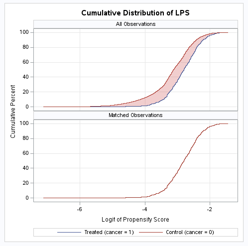
To complete the match, the matching algorithm was implemented in SAS. First, a PROC LOGISTIC was run using the covariates to generate the propensity score. The SAS PSMATCH routine then conducted the match. For this exercise, 1-1 greedy matching, nearest neighbor matching on the logit of the propensity score was performed. The PSMATCH routine produced Table 5 to aid with assessing matching performance. The table presents standardized mean differences for all observations, observations in the support region, and matched observations:
| Standardized Mean Differences (Treated – Control) | ||||||
|---|---|---|---|---|---|---|
| Variable | Observations | Mean Difference |
Standard Deviation |
Standardized Difference |
Percent Reduction |
Variance Ratio |
| Logit Prop Score | All | 0.45230 | 0.706286 | 0.64040 | 0.3692 | |
| Region | 0.42470 | 0.679118 | 0.62538 | 2.35 | 0.4118 | |
| Matched | 0.00001 | 0.518696 | 0.00001 | 100.00 | 1.0000 | |
| age_1165 | All | -0.12150 | 0.274892 | -0.44199 | 0.2018 | |
| Region | -0.11341 | 0.269594 | -0.42067 | 4.82 | 0.2115 | |
| Matched | -0.00200 | 0.162243 | -0.01233 | 97.21 | 0.9305 | |
| age70_74 | All | -0.00050 | 0.436791 | -0.00114 | 1.0006 | |
| Region | -0.00293 | 0.437466 | -0.00671 | 0.00 | 0.9945 | |
| Matched | 0.00000 | 0.438859 | 0.00000 | 100.00 | 1.0000 | |
| age75_79 | All | 0.05290 | 0.404920 | 0.13064 | 1.2109 | |
| Region | 0.05118 | 0.405595 | 0.12619 | 3.41 | 1.2021 | |
| Matched | -0.00600 | 0.425658 | -0.01410 | 89.21 | 0.9827 | |
| age80_84 | All | 0.03980 | 0.344632 | 0.11549 | 1.2788 | |
| Region | 0.03868 | 0.345251 | 0.11203 | 2.99 | 1.2684 | |
| Matched | 0.01000 | 0.360313 | 0.02775 | 75.97 | 1.0550 | |
| age_85plus | All | 0.05970 | 0.350184 | 0.17048 | 1.4224 | |
| Region | 0.05862 | 0.350780 | 0.16710 | 1.98 | 1.4108 | |
| Matched | -0.00200 | -0.380346 | -0.00526 | 96.92 | 0.9910 | |
| female | All | -0.10910 | 0.496459 | -0.21976 | 1.0276 | |
| Region | -0.10615 | 0.496701 | -0.21372 | 2.75 | 1.0255 | |
| Matched | -0.00200 | 0.499874 | -0.00400 | 98.18 | 0.9996 | |
| race_asian | All | -0.02590 | 0.193114 | -0.13412 | 0.5156 | |
| Region | -0.02488 | 0.191924 | -0.12963 | 3.35 | 0.5254 | |
| Matched | 0.00400 | 0.153189 | 0.02611 | 80.53 | 1.1770 | |
| race_black | All | -0.03980 | 0.319631 | -0.12452 | 0.7409 | |
| Region | -0.04109 | 0.320363 | -0.12826 | 0.00 | 0.7350 | |
| Matched | -0.00400 | 0.297606 | -0.01344 | 89.21 | 0.9643 | |
| race_hispanic | All | -0.04190 | 0.192392 | -0.21778 | 0.3145 | |
| Region | -0.03621 | 0.185725 | -0.19496 | 10.48 | 0.3454 | |
| Matched | -0.00200 | 0.136658 | -0.01464 | 93.28 | 0.9018 | |
| race_native_am | All | -0.00140 | 0.051908 | -0.02697 | 0.5902 | |
| Region | -0.00143 | 0.052062 | -0.02751 | 0.00 | 0.5847 | |
| Matched | -0.00200 | 0.054736 | -0.03654 | 0.00 | 0.5010 | |
| race_other | All | -0.00880 | 0.182286 | -0.04828 | 0.7818 | |
| Region | -0.00917 | 0.182751 | -0.05017 | 0.00 | 0.7747 | |
| Matched | 0.00000 | 0.170758 | 0.00000 | 100.00 | 1.0000 | |
| race_unk_miss | All | -0.01470 | 0.095976 | -0.15316 | 0.1218 | |
| Region | -0.01314 | 0.091963 | -0.14291 | 6.70 | 0.1341 | |
| Matched | 0.00200 | 0.031623 | 0.06325 | 58.71 | ||
| athhip | All | -0.03020 | 0.494684 | -0.06105 | 0.9840 | |
| Region | -0.02915 | 0.494622 | -0.05893 | 3.48 | 0.9845 | |
| Matched | 0.00600 | 0.492132 | 0.01219 | 80.03 | 1.0045 | |
| copd_e | All | -0.02910 | 0.381198 | -0.07634 | 0.8799 | |
| Region | -0.02748 | 0.380540 | -0.07222 | 5.40 | 0.8856 | |
| Matched | 0.01200 | 0.363169 | 0.03304 | 56.72 | 1.0648 | |
| sciatc | All | -0.03700 | 0.441964 | -0.08372 | 0.9169 | |
| Region | -0.03617 | 0.441762 | -0.08188 | 2.20 | 0.9186 | |
| Matched | 0.01200 | 0.428681 | 0.02799 | 66.56 | 1.0343 | |
| chf | All | -0.00550 | 0.284515 | -0.01933 | 0.9474 | |
| Region | -0.00516 | 0.284269 | -0.01814 | 6.16 | 0.9506 | |
| Matched | -0.00200 | 0.282116 | -0.00709 | 63.33 | 0.9794 | |
| stroke | All | 0.00840 | 0.277208 | 0.03030 | 1.0975 | |
| Region | 0.00835 | 0.277244 | 0.03012 | 0.59 | 1.0969 | |
| Matched | 0.00000 | 0.283579 | 0.00000 | 100.00 | 1.0000 | |
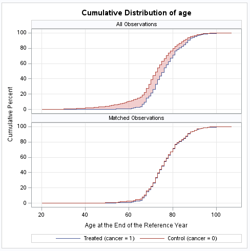
From Table 5, the covariates appear balanced after matching as no standardized differences are greater than 0.1 in the Matched rows, indicating the matching algorithm was successful. An examination of the cumulative distribution of the matching variable, the logit of propensity score, confirms the matching was successful as the distribution is now overlapping.
Software packages for matching and weighting
There are many software packages to aid investigators in matching and weighting. Several suggestions are presented in Table 6.
| Software | Algorithm | Command |
|---|---|---|
| SAS | Propensity Score Matching | PSMATCH |
| Coarsened Exact Matching | CEM |
|
| Stata | Propensity Score Matching | teffects psmatch |
| Coarsened Exact Matching | cem |
|
| Caliper Matching | calipmatch |
|
| R | All | MatchIt |
References
- Cook TD, Shadish WR, Wong VC. Three conditions under which experiments and observational studies produce comparable causal estimates: New findings from within‐study comparisons. Journal of Policy Analysis and Management: The Journal of the Association for Public Policy Analysis and Management. 2008;27(4):724-750.
- Caliendo M, Kopeinig S. Some practical guidance for the implementation of propensity score matching. Journal of economic surveys. 2008;22(1):31-72.
- Stuart EA. Matching methods for causal inference: A review and a look forward. Statistical science: a review journal of the Institute of Mathematical Statistics. 2010;25(1):1.
- Harris H, Horst SJ. A brief guide to decisions at each step of the propensity score matching process. Practical Assessment, Research, and Evaluation. 2016;21(1):4.
- Austin PC, Stuart EA. Moving towards best practice when using inverse probability of treatment weighting (IPTW) using the propensity score to estimate causal treatment effects in observational studies. Statistics in medicine. 2015;34(28):3661-3679.
- Li F, Morgan KL, Zaslavsky AM. Balancing covariates via propensity score weighting. Journal of the American Statistical Association. 2018;113(521):390-400.
- Iacus SM, King G, Porro G. Causal inference without balance checking: Coarsened exact matching. Political analysis. 2012;20(1):1-24.
- Reeve BB, Smith AW, Arora NK, Hays RD. Reducing bias in cancer research: application of propensity score matching. Health care financing review. 2008;29(4):69.
- Reeve BB, Stover AM, Jensen RE, et al. Impact of diagnosis and treatment of clinically localized prostate cancer on health‐related quality of life for older Americans: a population‐based study. Cancer. 2012;118(22):5679-5687.
- Leach CR, Bellizzi KM, Hurria A, Reeve BB. Is it my cancer or am i just getting older?: impact of cancer on age‐related health conditions of older cancer survivors. Cancer. 2016;122(12):1946-1953.
- Stover AM, Mayer DK, Muss H, Wheeler SB, Lyons JC, Reeve BB. Quality of life changes during the pre‐to postdiagnosis period and treatment‐related recovery time in older women with breast cancer. Cancer. 2014;120(12):1881-1889.
- Verma M, Paik JM, Younossi I, Tan D, Abdelaal H, Younossi ZM. The impact of hepatocellular carcinoma diagnosis on patients' health-related quality of life. Cancer Medicine. 2021;10(18):6273-6281.
- Lee E, Hines RB, Wright JL, Nam E, Rovito MJ, Liu X. Effects of Radiation Therapy and Comorbidity on Health-Related Quality of Life and Mortality Among Older Women With Low-Risk Breast Cancer: Protocol for a Retrospective Cohort Study. JMIR Res Protoc. 2020;9(11):e18056.
- Mahal AR, Cramer LD, Wang EH, et al. Did quality of life for older cancer survivors improve with the turn of the century in the United States? J Geriatr Oncol. 2021;12(1):102-105.
- Ali AA, Xiao H, Tawk R, et al. Comparison of health utility weights among elderly patients receiving breast-conserving surgery plus hormonal therapy with or without radiotherapy. Current Medical Research and Opinion. 2017;33(2):391-400.
- Rose S, Van der Laan MJ. Why match? Investigating matched case-control study designs with causal effect estimation. The international journal of biostatistics. 2009;5(1).
- Ali MS, Groenwold RH, Belitser SV, et al. Reporting of covariate selection and balance assessment in propensity score analysis is suboptimal: a systematic review. Journal of clinical epidemiology. 2015;68(2):122-131.
- Clauser SB, Arora NK, Bellizzi KM, Haffer SCC, Topor M, Hays RD. Disparities in HRQOL of cancer survivors and non-cancer managed care enrollees. Health care financing review. 2008;29(4):23.
- Kutner JS, Bryant LL, Beaty BL, Fairclough DL. Symptom distress and quality-of-life assessment at the end of life: the role of proxy response. Journal of pain and symptom management. 2006;32(4):300-310.
- Lapin BR, Thompson NR, Schuster A, Katzan IL. Patient versus proxy response on global health scales: No meaningful DIFference. Quality of Life Research. 2019;28(6):1585-1594.
- Kent EE, Ambs A, Mitchell SA, Clauser SB, Smith AW, Hays RD. Health‐related quality of life in older adult survivors of selected cancers: data from the SEER‐MHOS linkage. Cancer. 2015;121(5):758-765.
- Smith AW, Reeve BB, Bellizzi KM, et al. Cancer, comorbidities, and health-related quality of life of older adults. Health care financing review. 2008;29(4):41.
- Wang S-Y, Hsu SH, Gross CP, et al. Association between time since cancer diagnosis and health-related quality of life: a population-level analysis. Value in Health. 2016;19(5):631-638.
- Austin PC. Assessing covariate balance when using the generalized propensity score with quantitative or continuous exposures. Statistical methods in medical research. 2019;28(5):1365-1377.
- Zhang Z, Kim H, Lonjon G, Zhu Y. AME Big-Data Clinical Trial Collaborative Group. Balance diagnostics after propensity score matching. Ann Transl Med. 2019;7:16.
- Fullerton B, Pöhlmann B, Krohn R, Adams JL, Gerlach FM, Erler A. The Comparison of Matching Methods Using Different Measures of Balance: Benefits and Risks Exemplified within a Study to Evaluate the Effects of German Disease Management Programs on Long‐Term Outcomes of Patients with Type 2 Diabetes. Health services research. 2016;51(5):1960-1980.
- Nguyen T-L, Collins GS, Spence J, et al. Double-adjustment in propensity score matching analysis: choosing a threshold for considering residual imbalance. BMC medical research methodology. 2017;17(1):1-8.